Simulating the effect of data-splitting and stepwise selection on the lung dataset

This is Part Two of an four part series on model fitting and validation. Part One can be found here.

Introduction

The aim of this article is to consider the effect of using data-splitting (to obtain a single training and test set) and stepwise selection (to obtain ‘significant’ factors) on the lung R dataset.

In general – assuming we have data \(X \in \mathbb{R}^{n \times p}\) – the process consists of the following steps:

1. Randomly allocate the data to a training set, \(X_\text{train} \in \mathbb{R}^{n_1 \times p}\), and a test set, \(X_\text{test} \in \mathbb{R}^{n_2 \times p}\).
   • Here, \(n = n_1 + n_2\), where \(n_1 \approx 0.7 n\) and \(n_2 \approx 0.3 n\).
2. Perform model building on the test set, using stepwise selection starting with a model that includes all factors, to obtain model \(\mathcal{M}\).
   • Stepwise is performed by adding and removing a single factor at each step such that AIC is minimised. Here, \(\text{AIC} = 2k - 2 \log(\hat L)\), and \(\hat L\) is the maximised (partial) likelihood.
3. Perform model validation on the test set, to obtain Harrell’s C-index, assessing the predictive performance of the model over all observed times.
   • We are answering the question: Among all pairs of individuals, what fraction had predicted risks that were correctly ranked in the same order as their actual observed outcomes (event times)?

There are many issues with this procedure, which I have discussed in a previous post. In this article I will perform the above steps 100 times and obtain the following:

1. The amount of variability in the factors chosen in the model selection stage.
   • In addition, the variability in the coefficients estimated for each factor.
2. The amount of variability in the c-statistic obtained from validation on the test set.

Prerequisites and data cleaning

The lung dataset is from the {survival} package (Therneau 2024), and I will use {data.table} (Barrett et al. 2024) as I like the syntax and it’s fast.

Therneau, Terry M. 2024. A Package for Survival Analysis in r. https://CRAN.R-project.org/package=survival.

Barrett, Tyson, Matt Dowle, Arun Srinivasan, Jan Gorecki, Michael Chirico, Toby Hocking, and Benjamin Schwendinger. 2024. Data.table: Extension of ‘Data.frame‘. https://CRAN.R-project.org/package=data.table.

library(survival)
library(broom) # for 'tidy'
library(data.table)
options(datatable.print.nrows = 20) # set max # rows before truncating (default = 100)
library(ggplot2)
lung <- as.data.table(lung)
lung

      inst  time status   age   sex ph.ecog ph.karno pat.karno meal.cal wt.loss
     <num> <num>  <num> <num> <num>   <num>    <num>     <num>    <num>   <num>
  1:     3   306      2    74     1       1       90       100     1175      NA
  2:     3   455      2    68     1       0       90        90     1225      15
  3:     3  1010      1    56     1       0       90        90       NA      15
  4:     5   210      2    57     1       1       90        60     1150      11
  5:     1   883      2    60     1       0      100        90       NA       0
 ---                                                                           
224:     1   188      1    77     1       1       80        60       NA       3
225:    13   191      1    39     1       0       90        90     2350      -5
226:    32   105      1    75     2       2       60        70     1025       5
227:     6   174      1    66     1       1       90       100     1075       1
228:    22   177      1    58     2       1       80        90     1060       0

The lung dataset has status encoded in a non-standard way (as 1 for censored and 2 for dead). I will change this to 0 and 1 respectively. I will also ensure the data contains no missingness by using na.omit().

#recode 'status' as 1 if event and 0 if censored
lung_recode <- copy(lung)[, status := as.integer(status == 2)]

# remove NA's (st 'ampute' works)
lung_complete <- na.omit(lung_recode)

lung_complete[, `:=`(sex = as.factor(sex), ph.ecog = as.factor(ph.ecog))]

lung_complete

      inst  time status   age    sex ph.ecog ph.karno pat.karno meal.cal
     <num> <num>  <int> <num> <fctr>  <fctr>    <num>     <num>    <num>
  1:     3   455      1    68      1       0       90        90     1225
  2:     5   210      1    57      1       1       90        60     1150
  3:    12  1022      0    74      1       1       50        80      513
  4:     7   310      1    68      2       2       70        60      384
  5:    11   361      1    71      2       2       60        80      538
 ---                                                                    
163:    11   203      0    71      2       1       80        90     1025
164:    13   191      0    39      1       0       90        90     2350
165:    32   105      0    75      2       2       60        70     1025
166:     6   174      0    66      1       1       90       100     1075
167:    22   177      0    58      2       1       80        90     1060
     wt.loss
       <num>
  1:      15
  2:      11
  3:       0
  4:      10
  5:       1
 ---        
163:       0
164:      -5
165:       5
166:       1
167:       0

The code

Here, I’ll do the following:

• Randomly allocate \(\approx 70\%\) of the data to the training set, and the remainder to the test set.
• Use stepwise selection to choose ‘significant’ factors and estimate coefficients.
• Obtain the C-index on the test set.

For reproducibility, I’ll create a data.table where the rows consist of an .id variable – relating to the simulation number – and the row indices which will be chosen from lung_complete to make a training set for that simulation. This is shown in Listing 1.

set.seed(1000)

n_x <- nrow(lung_complete)
n1 <- 0.7 # size of training set

training_idx <- rbindlist(
                  lapply(seq_len(n_sim), function(i) {
                                idx <- sample(1:n_x, floor(n1 * n_x))
                                data.frame(.id = i, as.list(idx))
                                }
                        ),
                          use.names = FALSE
                  )

# change column names except '.id'
old_names <- names(training_idx)
new_names <- c(".id", paste0("idx_", seq_len(ncol(training_idx) - 1))) 
setnames(training_idx, old = old_names, new = new_names)

training_idx[1:5, 1:12]

Listing 1: Generating training set indices for data-splitting simulations

     .id idx_1 idx_2 idx_3 idx_4 idx_5 idx_6 idx_7 idx_8 idx_9 idx_10 idx_11
   <int> <int> <int> <int> <int> <int> <int> <int> <int> <int>  <int>  <int>
1:     1    68    43    51    88    29    99    61   146   150    102     45
2:     2   163    99   121    62     5   151   166    41     2    116    146
3:     3    40    52    26   101   133   102    71   119    13     32    166
4:     4   130   155    51   142    48    76    72    38    42     85     91
5:     5    37   126    87   166    59    93    14    84    74     49    110

Now, I’ll build 100 Cox proportional hazard models, using a stepwise procedure, on each training sample, and obtain the C-index on the respective test sample.

# split data into training and test sets
# and obtain cox coefs
models <- training_idx[, {
        tmp_train <- lung_complete[unlist(.SD)]
        tmp_test <- lung_complete[-unlist(.SD)]
        # fit the full model to the training data
        cox_full_tmp <- coxph(Surv(time, status) ~ .,
                              data = tmp_train)
        # use stepwise selection on training data
        cox_step_tmp <- step(cox_full_tmp,
                             direction = "both",
                             trace = 0)
        # get linear predictor on test data
        lp_tmp <- predict(cox_step_tmp, 
                          newdata = tmp_test, type = "lp")
        # obtain c-statistic using linear predictor
        # see callout note below for why `reverse = TRUE` is required
        c_stat <- concordance(Surv(tmp_test$time, tmp_test$status) ~ lp_tmp, 
                              reverse = TRUE) 
        data.table(as.data.table(tidy(cox_step_tmp)),
                         c = c_stat$concordance)
        }, by = .id] 
models 

Listing 2: Fitting Cox PH models on the training samples, and obtaining the C-index on the respective test samples

       .id     term    estimate  std.error statistic      p.value         c
     <int>   <char>       <num>      <num>     <num>        <num>     <num>
  1:     1     inst -0.02516878 0.01555328 -1.618230 1.056130e-01 0.5320829
  2:     1     sex2 -0.74073698 0.24700260 -2.998904 2.709530e-03 0.5320829
  3:     1 ph.ecog1  0.65422440 0.34366145  1.903689 5.695074e-02 0.5320829
  4:     1 ph.ecog2  1.94984289 0.52954389  3.682118 2.313046e-04 0.5320829
  5:     1 ph.ecog3  2.91211017 1.15977949  2.510917 1.204180e-02 0.5320829
 ---                                                                       
629:   100     sex2 -0.49918121 0.24386054 -2.046995 4.065862e-02 0.5729730
630:   100 ph.ecog1  0.90183824 0.31795471  2.836373 4.562908e-03 0.5729730
631:   100 ph.ecog2  2.66165163 0.57943576  4.593523 4.358245e-06 0.5729730
632:   100 ph.ecog3  3.61852274 1.17636760  3.076014 2.097883e-03 0.5729730
633:   100 ph.karno  0.04106388 0.01400488  2.932112 3.366650e-03 0.5729730

Calculating the C-statistic using concordance()

The reverse = TRUE argument in concordance() is important in Listing 2: if TRUE then assume that larger x values predict smaller response values y; a proportional hazards model is the common example of this, larger hazard = shorter survival.

The models output from Listing 2 has 7 columns. The .id variable refers back to the training sample obtained from training_idx in Listing 1, and the term variable gives the factors that have been selected in the model relating to the .id.¹ The c variable is the C-index obtained from using the .id\(^{\text{th}}\) model to predict the test set events, so is identical for rows with the same .id’s.

¹ The term estimates can contain NA’s if there is complete separation or zero events in the split.

Annoyingly, it appears to not be possible to both label / caption listings (using #| lst-label and #| lst-cap) and use code annotations (via # <1>). I’m not sure why, but worth remember for the future.

For example, if the code block contains the lines,

#| lst-cap: "An example of when the hover annotation doesn't work"
#| lst-label: lst-no-hover

then the output looks like this:

x <- rnorm(100)

Listing 3: An example of when the hover annotation doesn’t work

1

This hovering code annotation doesn’t work

Using the linear predictor to access predictive ability

Fitting a Cox proportional hazards model:

\[ \lambda(t \mid X) = \lambda_0(t) \exp(\beta_1 X_1 + \beta_2 X_2 + \dots + \beta_p X_p), \]

• \(\beta_1, \beta_2, \dots, \beta_p\) are the estimated coefficients.
  
• Linear Predictor: \[ \text{LP}(X) = \beta_1 X_1 + \beta_2 X_2 + \dots + \beta_p X_p. \]
• The hazard ratio between two individuals is determined by the difference in their linear predictors. A higher linear predictor implies a higher hazard (i.e., worse prognosis, or shorter survival on average).

Why the LP Is Enough to Rank Subjects

• Harrell’s c-index is fundamentally about whether the model places the higher risk on the patient who actually experiences the event earlier.
  
• In a Cox model, risk is monotonic in \(\exp(\text{LP})\). That is, if \(\text{LP}_A > \text{LP}_B\), then \(\exp(\text{LP}_A) > \exp(\text{LP}_B)\).
  
• So for pairwise comparisons, we only need to compare the linear predictor \(\text{LP}_A\) vs. \(\text{LP}_B\).
  
• If \(\text{LP}_A > \text{LP}_B\) but patient A actually survived longer, that pair is discordant. If A also died sooner, that pair is concordant.

Analysing the results

Using the models and coefficient estimates obtained in models (from Listing 2), I’ll look at a few things:

1. How often each factor is chosen – using the stepwise procedure – to be in the 100 models.
2. How many different models are chosen from the 100 stepwise selection procedures, and the proportion of times each model is selected.
3. The variability in the estimated factor coefficients (if there are chosen in the model).
4. The variability in the C-index obtained on the test set.

The model factors

First, let’s look at the proportion that each factor has been chosen to be in the 100 models.

which_variables <- models[, unique(term)]

proportion_variables <- rbindlist(
      lapply(1:length(which_variables), 
             function(i) {
              prop_tmp <- nrow(models[term == which_variables[i]]) / n_sim
              data.table(which_variables[i], prop_tmp)
                    }
             )
      )

# categorical factors in each model are present in the `models` dataset multiple times
# e.g. 'ph.ecog1', 'ph.ecog2', etc.
# create a "expl_factor" group by removing trailing digits
proportion_variables[
  , expl_factor := sub("[0-9]+$", "", V1)
]

# collapse by the explanatory factor
grouped_proportions <- proportion_variables[
  , .(prop = unique(prop_tmp)),
  by = expl_factor
]

grouped_proportions[order(prop, decreasing = TRUE)]

Listing 4: Obtaining the proportion that each factor is chosen to be in the models.

   expl_factor  prop
        <char> <num>
1:     ph.ecog  0.94
2:         sex  0.91
3:        inst  0.72
4:     wt.loss  0.68
5:    ph.karno  0.64
6:   pat.karno  0.30
7:         age  0.22
8:    meal.cal  0.04

Now I’ll consider each model and the factors obtained using the stepwise procedure. First – in Listing 5 – I’ll create a terms_string variable that gives a string containing all the terms in each of the 100 models. Then – in Listing 6 – I’ll group these models together to see how many different combination of factors have been chosen from the 100 stepwise selection procedures.

model_variables <- models[, .(
  terms_string = paste(
    unique(sub("[0-9]+$", "", term)),
    collapse = ", "
  )
), by = .id]

model_variables

Listing 5: Creating string of all the factors in each of the models.

       .id                                     terms_string
     <int>                                           <char>
  1:     1                     inst, sex, ph.ecog, ph.karno
  2:     2            inst, sex, ph.ecog, ph.karno, wt.loss
  3:     3                 sex, ph.ecog, pat.karno, wt.loss
  4:     4       sex, ph.ecog, ph.karno, pat.karno, wt.loss
  5:     5                inst, age, sex, ph.ecog, ph.karno
 ---                                                       
 96:    96             age, sex, ph.ecog, ph.karno, wt.loss
 97:    97            inst, sex, ph.ecog, ph.karno, wt.loss
 98:    98 inst, sex, ph.ecog, ph.karno, pat.karno, wt.loss
 99:    99                      age, sex, ph.ecog, ph.karno
100:   100                           sex, ph.ecog, ph.karno

Grouping these models together gives the follow:

proportion_model_variables <- model_variables[
      , .(prop = nrow(.SD) / nrow(model_variables))
      , by = terms_string]

#proportion_model_variables
proportion_model_variables[order(prop, decreasing = TRUE)]

Listing 6: Grouping models together to show the number of different models obtained from using stepwise selection.

                                        terms_string  prop
                                              <char> <num>
 1:            inst, sex, ph.ecog, ph.karno, wt.loss  0.14
 2:                      inst, sex, ph.ecog, wt.loss  0.13
 3: inst, sex, ph.ecog, ph.karno, pat.karno, wt.loss  0.11
 4:                     inst, sex, ph.ecog, ph.karno  0.06
 5:                inst, age, sex, ph.ecog, ph.karno  0.04
---                                                       
30:           inst, sex, ph.ecog, pat.karno, wt.loss  0.01
31:                                        pat.karno  0.01
32:                     inst, sex, ph.ecog, meal.cal  0.01
33:  inst, sex, ph.ecog, ph.karno, meal.cal, wt.loss  0.01
34:             age, sex, ph.ecog, ph.karno, wt.loss  0.01

That is, from 100 simulations of splitting the data into a training and test set, I’ve obtained 34 different models!

The factor coefficients

OK – let’s look at the variability of the coefficient estimates for each factor. First, I’ll get summary statistics for each factor coefficient. A box-plot showing this variability is given in Figure 1, and the kernel densities of the estimates are shown in Figure 2.

# Remove any rows that have NA in the estimate
models_clean <- subset(models, !is.na(estimate))

models_clean[, as.list(summary(estimate)), by = term]

         term          Min.       1st Qu.        Median          Mean
       <char>         <num>         <num>         <num>         <num>
 1:      inst -0.0509354446 -0.0365704124 -0.0302755030 -0.0320112247
 2:      sex2 -1.1315746564 -0.7029760419 -0.5881394025 -0.6093326104
 3:  ph.ecog1  0.1420228124  0.5092835045  0.7024669149  0.7242113000
 4:  ph.ecog2  0.8063634936  1.3599992736  1.7791183312  1.7739151854
 5:  ph.ecog3  1.8659038585  2.5201583000  3.0779479537  3.0501194170
 6:  ph.karno -0.0211069194  0.0252318873  0.0304998545  0.0305489979
 7:   wt.loss -0.0292142915 -0.0210200718 -0.0186741004 -0.0187607396
 8: pat.karno -0.0280318096 -0.0223547207 -0.0183404498 -0.0193037902
 9:       age  0.0208960667  0.0220780244  0.0227820171  0.0242739341
10:  meal.cal -0.0009556685 -0.0007011441 -0.0006010875 -0.0006590115
          3rd Qu.          Max.
            <num>         <num>
 1: -0.0262214394 -0.0216371920
 2: -0.5037040983 -0.3564017818
 3:  0.9017954598  1.4072391610
 4:  2.1107234044  2.8765227030
 5:  3.5501307812  4.2490415152
 6:  0.0372071507  0.0516899027
 7: -0.0160832211 -0.0122667120
 8: -0.0169197955 -0.0142537345
 9:  0.0248300821  0.0391007125
10: -0.0005589549 -0.0004782023

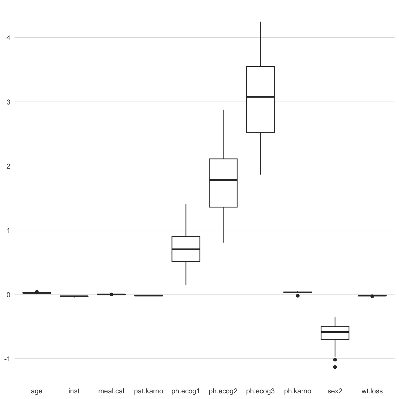
ggplot(models_clean, aes(x=term, y=estimate)) +
  geom_boxplot() +
  theme_minimal() +
  theme(
     axis.title = element_blank(),
     # remove the grid lines
     panel.grid.major = element_blank() ,
     panel.grid.minor = element_blank() ,
     # explicitly set the horizontal lines 
     panel.grid.major.y = element_line(linewidth = .1, color = "grey" )
        )

Figure 1: Box plots showing the variability in the factor coefficient estimates.

We can see from Figure 1 (and by referring back to Listing 4) that the factors that are chosen the most times have the largest varibility in their coefficient estimates.

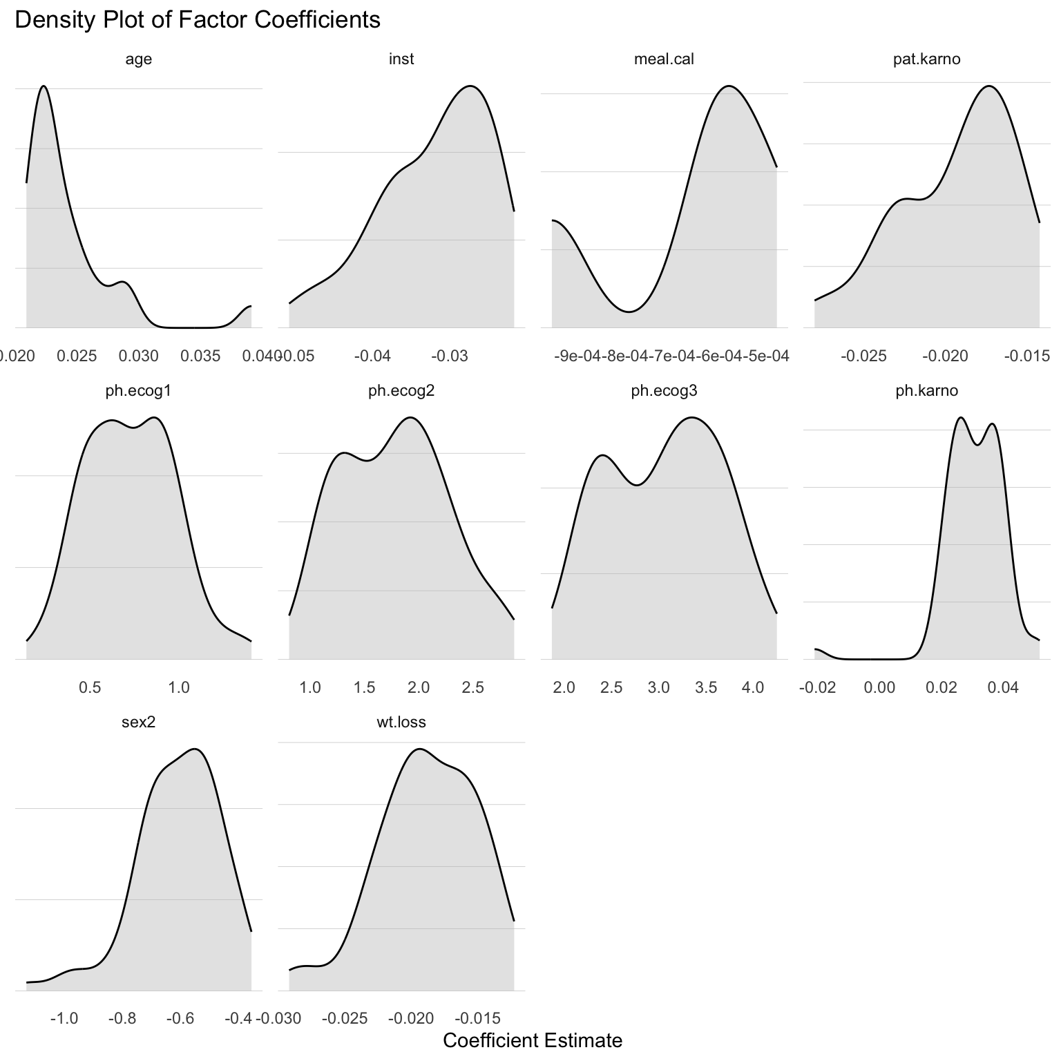
ggplot(models_clean, aes(x = estimate)) +
  geom_density(fill = "grey", alpha = 0.4) +
  facet_wrap(~ term, scales = "free") +
  labs(
    title = "Density Plot of Factor Coefficients",
    x = "Coefficient Estimate",
    y = "Density"
  ) +
  theme_minimal() +
  theme(
     axis.text.y = element_blank(),
     axis.title.y=element_blank(),
     # remove the grid lines
     panel.grid.major = element_blank() ,
     panel.grid.minor = element_blank() ,
     # explicitly set the horizontal lines 
     panel.grid.major.y = element_line(linewidth = .1, color = "grey" )
  )

Figure 2: Density plots of the estimates for each factor coefficient.

The C-Index on the test sets

Finally, let’s look at how the C-index varies for each training/test split and respective model. The code in Listing 7 gives the C-index values obtained from the 100 models, and the histogram is given in Figure 3.

c_stats <- models[, .(c_stats = unique(c)), by = .id]
c_stats[order(c_stats, decreasing = TRUE)]

Listing 7: Code to output the C-index, in descending order.

       .id   c_stats
     <int>     <num>
  1:    52 0.7121514
  2:     6 0.6835700
  3:    25 0.6673729
  4:    58 0.6621475
  5:    50 0.6596509
 ---                
 96:    53 0.5090000
 97:     7 0.5019802
 98:    18 0.4983819
 99:    66 0.4790356
100:     2 0.4610318

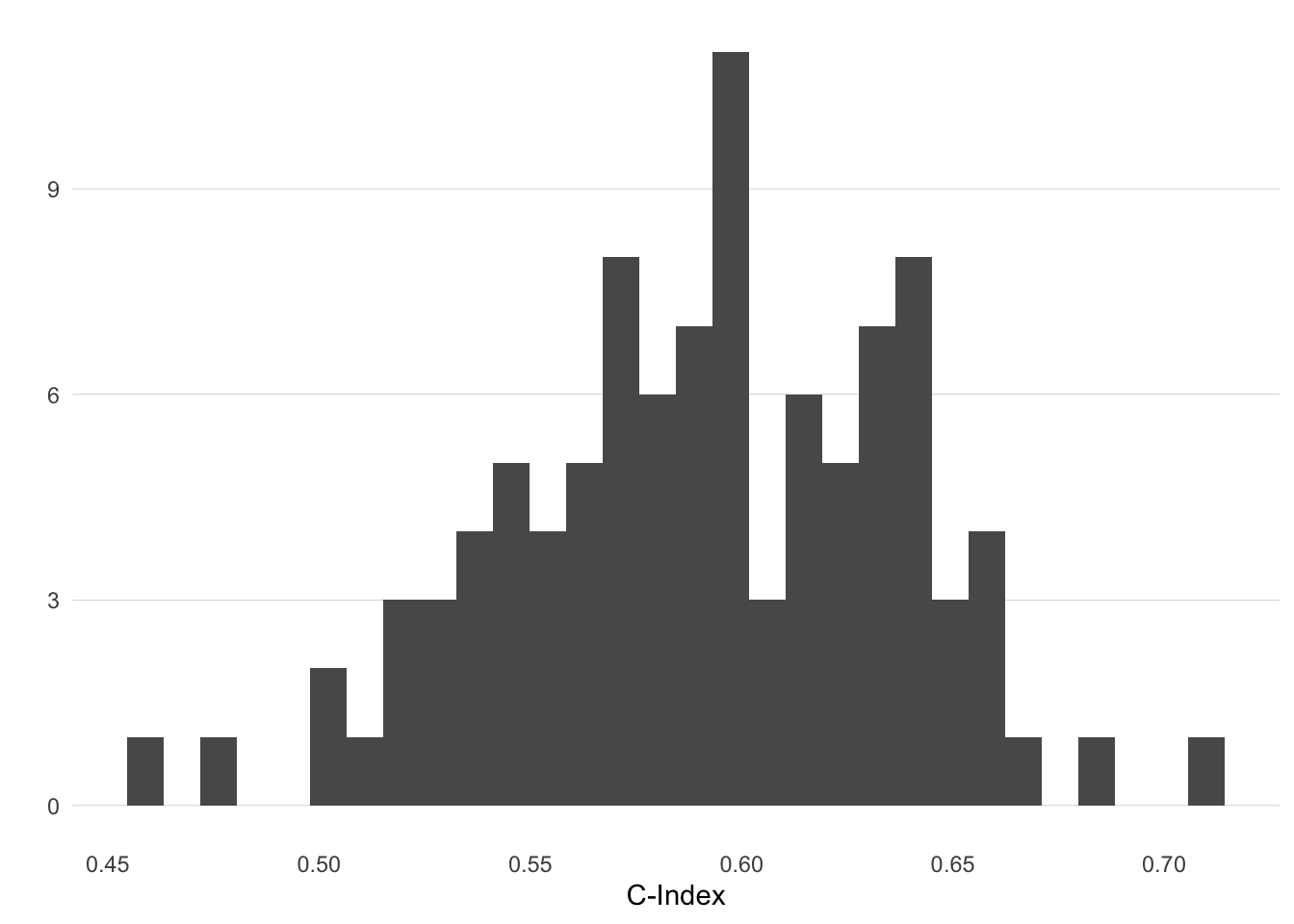
ggplot(c_stats, aes(x = c_stats)) +
        stat_bin(bins = 30) +
        xlab("C-Index") + ylab("") +
        theme_minimal() +
        theme(
           # remove the grid lines
           panel.grid.major = element_blank() ,
           panel.grid.minor = element_blank() ,
           # explicitly set the horizontal lines 
           panel.grid.major.y = element_line(linewidth = .1, color = "grey" )
        )

Figure 3: Histogram of the C-index values obtained on the test sets of the models.

These C-statistics varies quite a bit, from worse-than-random (a minimum of 0.46) to OK (a maximum of 0.71). Some of this variability could be accounted for by:

1. Some predictors might violate proportional hazards, hurting model performance.
2. Small test set size reduces the reliability of C-index estimates.

Conclusion

To sum up, I have shown by simulation some not-that-surprising results. These are:

• Building a model on a single training-test split and then performing stepwise selection creates a huge amount of variability, both in the model factors and in their coefficient estimates.
• The model validation step (performed on the test set) is not stable, and results in very different results depending on the data-split, the model and the coefficient estimates.

Next steps: I will examine better methods for model building and validation in some future posts, but as a spoiler, they will include the use of the lasso, bootstrapping and cross-validation.

Fin