library(mlr3)
library(mlr3viz)
library(mlr3learners)
library(mlr3tuning)
Loading required package: paradoxlibrary(mlr3tuningspaces)
library(ggplot2)
library(patchwork)
library(data.table)
options(datatable.print.nrows = 20)I am attempting to learn how to use {mlr3} (Lang et al. 2019), by reading through the book Applied Machine Learning Using mlr3 in R (Bischl et al. 2024).
In this post, I am working through the exercises given in Chapter 4 of the book (Becker, Schneider, and Fischer 2024), which covers hyperparameter optimisation (HPO). This includes the following:
regr.ranger on mtcars using random search and 3-fold CVspam using Brier score - Uses AutoTuner, predefined tuning spaces, and benchmark() for comparisonMy previous posts cover:
library(mlr3)
library(mlr3viz)
library(mlr3learners)
library(mlr3tuning)Loading required package: paradoxlibrary(mlr3tuningspaces)
library(ggplot2)
library(patchwork)
library(data.table)
options(datatable.print.nrows = 20)Suppress all messaging unless it’s a warning:1
1 The packages in {mlr3} that make use of optimization, i.e., {mlr3tuning} or {mlr3select}, use the logger of their base package {bbotk}.
lgr::get_logger("mlr3")$set_threshold("warn")
lgr::get_logger("bbotk")$set_threshold("warn")Tune the mtry, sample.fraction, and num.trees hyperparameters of lrn("regr.ranger") on tsk("mtcars"). Use a simple random search with 50 evaluations. Evaluate with a 3-fold CV and the root mean squared error. Visualize the effects that each hyperparameter has on the performance via simple marginal plots, which plot a single hyperparameter versus the cross-validated MSE.
Evaluate the performance of the model created in Exercise 1 with nested resampling. Use a holdout validation for the inner resampling and a 3-fold CV for the outer resampling.
Tune and benchmark an XGBoost model against a logistic regression (without tuning the latter) and determine which has the best Brier score. Use mlr3tuningspaces and nested resampling, try to pick appropriate inner and outer resampling strategies that balance computational efficiency vs. stability of the results.
(*) Write a function that implements an iterated random search procedure that drills down on the optimal configuration by applying random search to iteratively smaller search spaces. Your function should have seven inputs: task, learner, search_space, resampling, measure, random_search_stages, and random_search_size. You should only worry about programming this for fully numeric and bounded search spaces that have no dependencies. In pseudo-code:
 a. Create a random design of size `random_search_size` from the given search space and evaluate the learner on it.
 b. Identify the best configuration.
 c. Create a smaller search space around this best config, where you define the new range for each parameter as: `new_range[i] = (best_conf[i] - 0.25 * current_range[i], best_conf[i] + 0.25*current_range[i])`. Ensure that this `new_range` respects the initial bound of the original `search_space` by taking the `max()` of the new and old lower bound, and the `min()` of the new and the old upper bound (“clipping”).
d. Iterate the previous steps `random_search_stages` times and at the end return the best configuration you have ever evaluated. As a stretch goal, look into `mlr3tuning`’s internal source code and turn your function into an R6 class inheriting from the `TunerBatch` class – test it out on a learner of your choice.Tune the mtry, sample.fraction, and num.trees hyperparameters of lrn("regr.ranger") on tsk("mtcars"). Use a simple random search with 50 evaluations. Evaluate with a 3-fold CV and the root mean squared error. Visualize the effects that each hyperparameter has on the performance via simple marginal plots, which plot a single hyperparameter versus the cross-validated MSE.
Let’s load the task and look at the properties of the mtry, sample.fraction, and num.trees parameters.
tsk_mtcars <- tsk("mtcars")
lrn("regr.ranger")$param_set$data[id %in% c("mtry", "sample.fraction", "num.trees")]
id class lower upper levels nlevels is_bounded special_vals
<char> <char> <num> <num> <list> <num> <lgcl> <list>
1: mtry ParamInt 1 Inf [NULL] Inf FALSE <list[1]>
2: num.trees ParamInt 1 Inf [NULL] Inf FALSE <list[0]>
3: sample.fraction ParamDbl 0 1 [NULL] Inf TRUE <list[0]>
default storage_type tags
<list> <char> <list>
1: <NoDefault[0]> integer train
2: 500 integer train,predict,hotstart
3: <NoDefault[0]> numeric trainThe hyperparameters I’m looking at are:
mtry: number of variables considered at each tree split.num.trees: number of trees in the forest.sample.fraction: fraction of observations used to train each tree.Now I will set up the tuning of the mtry, sample.fraction, and num.trees hyperparameters.
learner <- lrn("regr.ranger",
               mtry = to_tune(p_int(1, 10)),
               num.trees = to_tune(20, 2000),
               sample.fraction = to_tune(0.1, 1))
learner
── <LearnerRegrRanger> (regr.ranger): Random Forest ────────────────────────────
• Model: -
• Parameters: mtry=<ObjectTuneToken>, num.threads=1,
num.trees=<RangeTuneToken>, sample.fraction=<RangeTuneToken>
• Packages: mlr3, mlr3learners, and ranger
• Predict Types: [response], se, and quantiles
• Feature Types: logical, integer, numeric, character, factor, and ordered
• Encapsulation: none (fallback: -)
• Properties: hotstart_backward, importance, missings, oob_error,
selected_features, and weights
• Other settings: use_weights = 'use'
Setting up an instance to terminate the tuner after 50 evaluations, and to use 3-fold CV.
instance <- ti(task = tsk_mtcars,
               learner = learner,
               resampling = rsmp("cv", folds = 3),
               # rmse gives interpretability in the original units (MPG) rather than squared units
               measures = msr("regr.rmse"),
               terminator = trm("evals", n_evals = 50))
instance
── <TuningInstanceBatchSingleCrit> ─────────────────────────────────────────────
• State: Not optimized
• Objective: <ObjectiveTuningBatch>
• Search Space:
                id    class lower upper nlevels
            <char>   <char> <num> <num>   <num>
1:            mtry ParamInt   1.0    10      10
2:       num.trees ParamInt  20.0  2000    1981
3: sample.fraction ParamDbl   0.1     1     Inf
• Terminator: <TerminatorEvals> (n_evals=50, k=0)
The tuning step uses 3-fold cross-validation:
Now I can set up the tuning process (random search).
tuner <- tnr("random_search")
#tuner$param_set
tuner
<TunerBatchRandomSearch>: Random Search
* Parameters: batch_size=1
* Parameter classes: ParamLgl, ParamInt, ParamDbl, ParamFct
* Properties: dependencies, single-crit, multi-crit
* Packages: mlr3tuning, bbotkAnd trigger the tuning process.
set.seed(333)
tuner$optimize(instance)
Warning in .__Task__weights(self = self, private = private, super = super, : 'Task$weights' is deprecated.
Use 'Task$weights_learner' instead.
See help("Deprecated")
Warning in .__Task__weights(self = self, private = private, super = super, : 'Task$weights' is deprecated.
Use 'Task$weights_learner' instead.
See help("Deprecated")
Warning in .__Task__weights(self = self, private = private, super = super, : 'Task$weights' is deprecated.
Use 'Task$weights_learner' instead.
See help("Deprecated")
Warning in .__Task__weights(self = self, private = private, super = super, : 'Task$weights' is deprecated.
Use 'Task$weights_learner' instead.
See help("Deprecated")
Warning in .__Task__weights(self = self, private = private, super = super, : 'Task$weights' is deprecated.
Use 'Task$weights_learner' instead.
See help("Deprecated")
Warning in .__Task__weights(self = self, private = private, super = super, : 'Task$weights' is deprecated.
Use 'Task$weights_learner' instead.
See help("Deprecated")
Warning in .__Task__weights(self = self, private = private, super = super, : 'Task$weights' is deprecated.
Use 'Task$weights_learner' instead.
See help("Deprecated")
Warning in .__Task__weights(self = self, private = private, super = super, : 'Task$weights' is deprecated.
Use 'Task$weights_learner' instead.
See help("Deprecated")
Warning in .__Task__weights(self = self, private = private, super = super, : 'Task$weights' is deprecated.
Use 'Task$weights_learner' instead.
See help("Deprecated")
Warning in .__Task__weights(self = self, private = private, super = super, : 'Task$weights' is deprecated.
Use 'Task$weights_learner' instead.
See help("Deprecated")
Warning in .__Task__weights(self = self, private = private, super = super, : 'Task$weights' is deprecated.
Use 'Task$weights_learner' instead.
See help("Deprecated")
Warning in .__Task__weights(self = self, private = private, super = super, : 'Task$weights' is deprecated.
Use 'Task$weights_learner' instead.
See help("Deprecated")
Warning in .__Task__weights(self = self, private = private, super = super, : 'Task$weights' is deprecated.
Use 'Task$weights_learner' instead.
See help("Deprecated")
Warning in .__Task__weights(self = self, private = private, super = super, : 'Task$weights' is deprecated.
Use 'Task$weights_learner' instead.
See help("Deprecated")
Warning in .__Task__weights(self = self, private = private, super = super, : 'Task$weights' is deprecated.
Use 'Task$weights_learner' instead.
See help("Deprecated")
Warning in .__Task__weights(self = self, private = private, super = super, : 'Task$weights' is deprecated.
Use 'Task$weights_learner' instead.
See help("Deprecated")
Warning in .__Task__weights(self = self, private = private, super = super, : 'Task$weights' is deprecated.
Use 'Task$weights_learner' instead.
See help("Deprecated")
Warning in .__Task__weights(self = self, private = private, super = super, : 'Task$weights' is deprecated.
Use 'Task$weights_learner' instead.
See help("Deprecated")
Warning in .__Task__weights(self = self, private = private, super = super, : 'Task$weights' is deprecated.
Use 'Task$weights_learner' instead.
See help("Deprecated")
Warning in .__Task__weights(self = self, private = private, super = super, : 'Task$weights' is deprecated.
Use 'Task$weights_learner' instead.
See help("Deprecated")
Warning in .__Task__weights(self = self, private = private, super = super, : 'Task$weights' is deprecated.
Use 'Task$weights_learner' instead.
See help("Deprecated")
Warning in .__Task__weights(self = self, private = private, super = super, : 'Task$weights' is deprecated.
Use 'Task$weights_learner' instead.
See help("Deprecated")
Warning in .__Task__weights(self = self, private = private, super = super, : 'Task$weights' is deprecated.
Use 'Task$weights_learner' instead.
See help("Deprecated")
Warning in .__Task__weights(self = self, private = private, super = super, : 'Task$weights' is deprecated.
Use 'Task$weights_learner' instead.
See help("Deprecated")
Warning in .__Task__weights(self = self, private = private, super = super, : 'Task$weights' is deprecated.
Use 'Task$weights_learner' instead.
See help("Deprecated")
Warning in .__Task__weights(self = self, private = private, super = super, : 'Task$weights' is deprecated.
Use 'Task$weights_learner' instead.
See help("Deprecated")
Warning in .__Task__weights(self = self, private = private, super = super, : 'Task$weights' is deprecated.
Use 'Task$weights_learner' instead.
See help("Deprecated")
Warning in .__Task__weights(self = self, private = private, super = super, : 'Task$weights' is deprecated.
Use 'Task$weights_learner' instead.
See help("Deprecated")
Warning in .__Task__weights(self = self, private = private, super = super, : 'Task$weights' is deprecated.
Use 'Task$weights_learner' instead.
See help("Deprecated")
Warning in .__Task__weights(self = self, private = private, super = super, : 'Task$weights' is deprecated.
Use 'Task$weights_learner' instead.
See help("Deprecated")
Warning in .__Task__weights(self = self, private = private, super = super, : 'Task$weights' is deprecated.
Use 'Task$weights_learner' instead.
See help("Deprecated")
Warning in .__Task__weights(self = self, private = private, super = super, : 'Task$weights' is deprecated.
Use 'Task$weights_learner' instead.
See help("Deprecated")
Warning in .__Task__weights(self = self, private = private, super = super, : 'Task$weights' is deprecated.
Use 'Task$weights_learner' instead.
See help("Deprecated")
Warning in .__Task__weights(self = self, private = private, super = super, : 'Task$weights' is deprecated.
Use 'Task$weights_learner' instead.
See help("Deprecated")
Warning in .__Task__weights(self = self, private = private, super = super, : 'Task$weights' is deprecated.
Use 'Task$weights_learner' instead.
See help("Deprecated")
Warning in .__Task__weights(self = self, private = private, super = super, : 'Task$weights' is deprecated.
Use 'Task$weights_learner' instead.
See help("Deprecated")
Warning in .__Task__weights(self = self, private = private, super = super, : 'Task$weights' is deprecated.
Use 'Task$weights_learner' instead.
See help("Deprecated")
Warning in .__Task__weights(self = self, private = private, super = super, : 'Task$weights' is deprecated.
Use 'Task$weights_learner' instead.
See help("Deprecated")
Warning in .__Task__weights(self = self, private = private, super = super, : 'Task$weights' is deprecated.
Use 'Task$weights_learner' instead.
See help("Deprecated")
Warning in .__Task__weights(self = self, private = private, super = super, : 'Task$weights' is deprecated.
Use 'Task$weights_learner' instead.
See help("Deprecated")
Warning in .__Task__weights(self = self, private = private, super = super, : 'Task$weights' is deprecated.
Use 'Task$weights_learner' instead.
See help("Deprecated")
Warning in .__Task__weights(self = self, private = private, super = super, : 'Task$weights' is deprecated.
Use 'Task$weights_learner' instead.
See help("Deprecated")
Warning in .__Task__weights(self = self, private = private, super = super, : 'Task$weights' is deprecated.
Use 'Task$weights_learner' instead.
See help("Deprecated")
Warning in .__Task__weights(self = self, private = private, super = super, : 'Task$weights' is deprecated.
Use 'Task$weights_learner' instead.
See help("Deprecated")
Warning in .__Task__weights(self = self, private = private, super = super, : 'Task$weights' is deprecated.
Use 'Task$weights_learner' instead.
See help("Deprecated")
Warning in .__Task__weights(self = self, private = private, super = super, : 'Task$weights' is deprecated.
Use 'Task$weights_learner' instead.
See help("Deprecated")
Warning in .__Task__weights(self = self, private = private, super = super, : 'Task$weights' is deprecated.
Use 'Task$weights_learner' instead.
See help("Deprecated")
Warning in .__Task__weights(self = self, private = private, super = super, : 'Task$weights' is deprecated.
Use 'Task$weights_learner' instead.
See help("Deprecated")
Warning in .__Task__weights(self = self, private = private, super = super, : 'Task$weights' is deprecated.
Use 'Task$weights_learner' instead.
See help("Deprecated")
Warning in .__Task__weights(self = self, private = private, super = super, : 'Task$weights' is deprecated.
Use 'Task$weights_learner' instead.
See help("Deprecated")
Warning in .__Task__weights(self = self, private = private, super = super, : 'Task$weights' is deprecated.
Use 'Task$weights_learner' instead.
See help("Deprecated")
Warning in .__Task__weights(self = self, private = private, super = super, : 'Task$weights' is deprecated.
Use 'Task$weights_learner' instead.
See help("Deprecated")
Warning in .__Task__weights(self = self, private = private, super = super, : 'Task$weights' is deprecated.
Use 'Task$weights_learner' instead.
See help("Deprecated")
Warning in .__Task__weights(self = self, private = private, super = super, : 'Task$weights' is deprecated.
Use 'Task$weights_learner' instead.
See help("Deprecated")
Warning in .__Task__weights(self = self, private = private, super = super, : 'Task$weights' is deprecated.
Use 'Task$weights_learner' instead.
See help("Deprecated")
Warning in .__Task__weights(self = self, private = private, super = super, : 'Task$weights' is deprecated.
Use 'Task$weights_learner' instead.
See help("Deprecated")
Warning in .__Task__weights(self = self, private = private, super = super, : 'Task$weights' is deprecated.
Use 'Task$weights_learner' instead.
See help("Deprecated")
Warning in .__Task__weights(self = self, private = private, super = super, : 'Task$weights' is deprecated.
Use 'Task$weights_learner' instead.
See help("Deprecated")
Warning in .__Task__weights(self = self, private = private, super = super, : 'Task$weights' is deprecated.
Use 'Task$weights_learner' instead.
See help("Deprecated")
Warning in .__Task__weights(self = self, private = private, super = super, : 'Task$weights' is deprecated.
Use 'Task$weights_learner' instead.
See help("Deprecated")
Warning in .__Task__weights(self = self, private = private, super = super, : 'Task$weights' is deprecated.
Use 'Task$weights_learner' instead.
See help("Deprecated")
Warning in .__Task__weights(self = self, private = private, super = super, : 'Task$weights' is deprecated.
Use 'Task$weights_learner' instead.
See help("Deprecated")
Warning in .__Task__weights(self = self, private = private, super = super, : 'Task$weights' is deprecated.
Use 'Task$weights_learner' instead.
See help("Deprecated")
Warning in .__Task__weights(self = self, private = private, super = super, : 'Task$weights' is deprecated.
Use 'Task$weights_learner' instead.
See help("Deprecated")
Warning in .__Task__weights(self = self, private = private, super = super, : 'Task$weights' is deprecated.
Use 'Task$weights_learner' instead.
See help("Deprecated")
Warning in .__Task__weights(self = self, private = private, super = super, : 'Task$weights' is deprecated.
Use 'Task$weights_learner' instead.
See help("Deprecated")
Warning in .__Task__weights(self = self, private = private, super = super, : 'Task$weights' is deprecated.
Use 'Task$weights_learner' instead.
See help("Deprecated")
Warning in .__Task__weights(self = self, private = private, super = super, : 'Task$weights' is deprecated.
Use 'Task$weights_learner' instead.
See help("Deprecated")
Warning in .__Task__weights(self = self, private = private, super = super, : 'Task$weights' is deprecated.
Use 'Task$weights_learner' instead.
See help("Deprecated")
Warning in .__Task__weights(self = self, private = private, super = super, : 'Task$weights' is deprecated.
Use 'Task$weights_learner' instead.
See help("Deprecated")
Warning in .__Task__weights(self = self, private = private, super = super, : 'Task$weights' is deprecated.
Use 'Task$weights_learner' instead.
See help("Deprecated")
Warning in .__Task__weights(self = self, private = private, super = super, : 'Task$weights' is deprecated.
Use 'Task$weights_learner' instead.
See help("Deprecated")
Warning in .__Task__weights(self = self, private = private, super = super, : 'Task$weights' is deprecated.
Use 'Task$weights_learner' instead.
See help("Deprecated")
Warning in .__Task__weights(self = self, private = private, super = super, : 'Task$weights' is deprecated.
Use 'Task$weights_learner' instead.
See help("Deprecated")
Warning in .__Task__weights(self = self, private = private, super = super, : 'Task$weights' is deprecated.
Use 'Task$weights_learner' instead.
See help("Deprecated")
Warning in .__Task__weights(self = self, private = private, super = super, : 'Task$weights' is deprecated.
Use 'Task$weights_learner' instead.
See help("Deprecated")
Warning in .__Task__weights(self = self, private = private, super = super, : 'Task$weights' is deprecated.
Use 'Task$weights_learner' instead.
See help("Deprecated")
Warning in .__Task__weights(self = self, private = private, super = super, : 'Task$weights' is deprecated.
Use 'Task$weights_learner' instead.
See help("Deprecated")
Warning in .__Task__weights(self = self, private = private, super = super, : 'Task$weights' is deprecated.
Use 'Task$weights_learner' instead.
See help("Deprecated")
Warning in .__Task__weights(self = self, private = private, super = super, : 'Task$weights' is deprecated.
Use 'Task$weights_learner' instead.
See help("Deprecated")
Warning in .__Task__weights(self = self, private = private, super = super, : 'Task$weights' is deprecated.
Use 'Task$weights_learner' instead.
See help("Deprecated")
Warning in .__Task__weights(self = self, private = private, super = super, : 'Task$weights' is deprecated.
Use 'Task$weights_learner' instead.
See help("Deprecated")
Warning in .__Task__weights(self = self, private = private, super = super, : 'Task$weights' is deprecated.
Use 'Task$weights_learner' instead.
See help("Deprecated")
Warning in .__Task__weights(self = self, private = private, super = super, : 'Task$weights' is deprecated.
Use 'Task$weights_learner' instead.
See help("Deprecated")
Warning in .__Task__weights(self = self, private = private, super = super, : 'Task$weights' is deprecated.
Use 'Task$weights_learner' instead.
See help("Deprecated")
Warning in .__Task__weights(self = self, private = private, super = super, : 'Task$weights' is deprecated.
Use 'Task$weights_learner' instead.
See help("Deprecated")
Warning in .__Task__weights(self = self, private = private, super = super, : 'Task$weights' is deprecated.
Use 'Task$weights_learner' instead.
See help("Deprecated")
Warning in .__Task__weights(self = self, private = private, super = super, : 'Task$weights' is deprecated.
Use 'Task$weights_learner' instead.
See help("Deprecated")
Warning in .__Task__weights(self = self, private = private, super = super, : 'Task$weights' is deprecated.
Use 'Task$weights_learner' instead.
See help("Deprecated")
Warning in .__Task__weights(self = self, private = private, super = super, : 'Task$weights' is deprecated.
Use 'Task$weights_learner' instead.
See help("Deprecated")
Warning in .__Task__weights(self = self, private = private, super = super, : 'Task$weights' is deprecated.
Use 'Task$weights_learner' instead.
See help("Deprecated")
Warning in .__Task__weights(self = self, private = private, super = super, : 'Task$weights' is deprecated.
Use 'Task$weights_learner' instead.
See help("Deprecated")
Warning in .__Task__weights(self = self, private = private, super = super, : 'Task$weights' is deprecated.
Use 'Task$weights_learner' instead.
See help("Deprecated")
Warning in .__Task__weights(self = self, private = private, super = super, : 'Task$weights' is deprecated.
Use 'Task$weights_learner' instead.
See help("Deprecated")
Warning in .__Task__weights(self = self, private = private, super = super, : 'Task$weights' is deprecated.
Use 'Task$weights_learner' instead.
See help("Deprecated")
Warning in .__Task__weights(self = self, private = private, super = super, : 'Task$weights' is deprecated.
Use 'Task$weights_learner' instead.
See help("Deprecated")
Warning in .__Task__weights(self = self, private = private, super = super, : 'Task$weights' is deprecated.
Use 'Task$weights_learner' instead.
See help("Deprecated")
Warning in .__Task__weights(self = self, private = private, super = super, : 'Task$weights' is deprecated.
Use 'Task$weights_learner' instead.
See help("Deprecated")
Warning in .__Task__weights(self = self, private = private, super = super, : 'Task$weights' is deprecated.
Use 'Task$weights_learner' instead.
See help("Deprecated")
Warning in .__Task__weights(self = self, private = private, super = super, : 'Task$weights' is deprecated.
Use 'Task$weights_learner' instead.
See help("Deprecated")
Warning in .__Task__weights(self = self, private = private, super = super, : 'Task$weights' is deprecated.
Use 'Task$weights_learner' instead.
See help("Deprecated")
Warning in .__Task__weights(self = self, private = private, super = super, : 'Task$weights' is deprecated.
Use 'Task$weights_learner' instead.
See help("Deprecated")
Warning in .__Task__weights(self = self, private = private, super = super, : 'Task$weights' is deprecated.
Use 'Task$weights_learner' instead.
See help("Deprecated")
Warning in .__Task__weights(self = self, private = private, super = super, : 'Task$weights' is deprecated.
Use 'Task$weights_learner' instead.
See help("Deprecated")
Warning in .__Task__weights(self = self, private = private, super = super, : 'Task$weights' is deprecated.
Use 'Task$weights_learner' instead.
See help("Deprecated")
Warning in .__Task__weights(self = self, private = private, super = super, : 'Task$weights' is deprecated.
Use 'Task$weights_learner' instead.
See help("Deprecated")
Warning in .__Task__weights(self = self, private = private, super = super, : 'Task$weights' is deprecated.
Use 'Task$weights_learner' instead.
See help("Deprecated")
Warning in .__Task__weights(self = self, private = private, super = super, : 'Task$weights' is deprecated.
Use 'Task$weights_learner' instead.
See help("Deprecated")
Warning in .__Task__weights(self = self, private = private, super = super, : 'Task$weights' is deprecated.
Use 'Task$weights_learner' instead.
See help("Deprecated")
Warning in .__Task__weights(self = self, private = private, super = super, : 'Task$weights' is deprecated.
Use 'Task$weights_learner' instead.
See help("Deprecated")
Warning in .__Task__weights(self = self, private = private, super = super, : 'Task$weights' is deprecated.
Use 'Task$weights_learner' instead.
See help("Deprecated")
Warning in .__Task__weights(self = self, private = private, super = super, : 'Task$weights' is deprecated.
Use 'Task$weights_learner' instead.
See help("Deprecated")
Warning in .__Task__weights(self = self, private = private, super = super, : 'Task$weights' is deprecated.
Use 'Task$weights_learner' instead.
See help("Deprecated")
Warning in .__Task__weights(self = self, private = private, super = super, : 'Task$weights' is deprecated.
Use 'Task$weights_learner' instead.
See help("Deprecated")
Warning in .__Task__weights(self = self, private = private, super = super, : 'Task$weights' is deprecated.
Use 'Task$weights_learner' instead.
See help("Deprecated")
Warning in .__Task__weights(self = self, private = private, super = super, : 'Task$weights' is deprecated.
Use 'Task$weights_learner' instead.
See help("Deprecated")
Warning in .__Task__weights(self = self, private = private, super = super, : 'Task$weights' is deprecated.
Use 'Task$weights_learner' instead.
See help("Deprecated")
Warning in .__Task__weights(self = self, private = private, super = super, : 'Task$weights' is deprecated.
Use 'Task$weights_learner' instead.
See help("Deprecated")
Warning in .__Task__weights(self = self, private = private, super = super, : 'Task$weights' is deprecated.
Use 'Task$weights_learner' instead.
See help("Deprecated")
Warning in .__Task__weights(self = self, private = private, super = super, : 'Task$weights' is deprecated.
Use 'Task$weights_learner' instead.
See help("Deprecated")
Warning in .__Task__weights(self = self, private = private, super = super, : 'Task$weights' is deprecated.
Use 'Task$weights_learner' instead.
See help("Deprecated")
Warning in .__Task__weights(self = self, private = private, super = super, : 'Task$weights' is deprecated.
Use 'Task$weights_learner' instead.
See help("Deprecated")
Warning in .__Task__weights(self = self, private = private, super = super, : 'Task$weights' is deprecated.
Use 'Task$weights_learner' instead.
See help("Deprecated")
Warning in .__Task__weights(self = self, private = private, super = super, : 'Task$weights' is deprecated.
Use 'Task$weights_learner' instead.
See help("Deprecated")
Warning in .__Task__weights(self = self, private = private, super = super, : 'Task$weights' is deprecated.
Use 'Task$weights_learner' instead.
See help("Deprecated")
Warning in .__Task__weights(self = self, private = private, super = super, : 'Task$weights' is deprecated.
Use 'Task$weights_learner' instead.
See help("Deprecated")
Warning in .__Task__weights(self = self, private = private, super = super, : 'Task$weights' is deprecated.
Use 'Task$weights_learner' instead.
See help("Deprecated")
Warning in .__Task__weights(self = self, private = private, super = super, : 'Task$weights' is deprecated.
Use 'Task$weights_learner' instead.
See help("Deprecated")
Warning in .__Task__weights(self = self, private = private, super = super, : 'Task$weights' is deprecated.
Use 'Task$weights_learner' instead.
See help("Deprecated")
Warning in .__Task__weights(self = self, private = private, super = super, : 'Task$weights' is deprecated.
Use 'Task$weights_learner' instead.
See help("Deprecated")
Warning in .__Task__weights(self = self, private = private, super = super, : 'Task$weights' is deprecated.
Use 'Task$weights_learner' instead.
See help("Deprecated")
Warning in .__Task__weights(self = self, private = private, super = super, : 'Task$weights' is deprecated.
Use 'Task$weights_learner' instead.
See help("Deprecated")
Warning in .__Task__weights(self = self, private = private, super = super, : 'Task$weights' is deprecated.
Use 'Task$weights_learner' instead.
See help("Deprecated")
Warning in .__Task__weights(self = self, private = private, super = super, : 'Task$weights' is deprecated.
Use 'Task$weights_learner' instead.
See help("Deprecated")
Warning in .__Task__weights(self = self, private = private, super = super, : 'Task$weights' is deprecated.
Use 'Task$weights_learner' instead.
See help("Deprecated")
Warning in .__Task__weights(self = self, private = private, super = super, : 'Task$weights' is deprecated.
Use 'Task$weights_learner' instead.
See help("Deprecated")
Warning in .__Task__weights(self = self, private = private, super = super, : 'Task$weights' is deprecated.
Use 'Task$weights_learner' instead.
See help("Deprecated")
Warning in .__Task__weights(self = self, private = private, super = super, : 'Task$weights' is deprecated.
Use 'Task$weights_learner' instead.
See help("Deprecated")
Warning in .__Task__weights(self = self, private = private, super = super, : 'Task$weights' is deprecated.
Use 'Task$weights_learner' instead.
See help("Deprecated")
Warning in .__Task__weights(self = self, private = private, super = super, : 'Task$weights' is deprecated.
Use 'Task$weights_learner' instead.
See help("Deprecated")
Warning in .__Task__weights(self = self, private = private, super = super, : 'Task$weights' is deprecated.
Use 'Task$weights_learner' instead.
See help("Deprecated")
Warning in .__Task__weights(self = self, private = private, super = super, : 'Task$weights' is deprecated.
Use 'Task$weights_learner' instead.
See help("Deprecated")
Warning in .__Task__weights(self = self, private = private, super = super, : 'Task$weights' is deprecated.
Use 'Task$weights_learner' instead.
See help("Deprecated")
Warning in .__Task__weights(self = self, private = private, super = super, : 'Task$weights' is deprecated.
Use 'Task$weights_learner' instead.
See help("Deprecated")
Warning in .__Task__weights(self = self, private = private, super = super, : 'Task$weights' is deprecated.
Use 'Task$weights_learner' instead.
See help("Deprecated")
Warning in .__Task__weights(self = self, private = private, super = super, : 'Task$weights' is deprecated.
Use 'Task$weights_learner' instead.
See help("Deprecated")
Warning in .__Task__weights(self = self, private = private, super = super, : 'Task$weights' is deprecated.
Use 'Task$weights_learner' instead.
See help("Deprecated")
Warning in .__Task__weights(self = self, private = private, super = super, : 'Task$weights' is deprecated.
Use 'Task$weights_learner' instead.
See help("Deprecated")
Warning in .__Task__weights(self = self, private = private, super = super, : 'Task$weights' is deprecated.
Use 'Task$weights_learner' instead.
See help("Deprecated")
Warning in .__Task__weights(self = self, private = private, super = super, : 'Task$weights' is deprecated.
Use 'Task$weights_learner' instead.
See help("Deprecated") mtry num.trees sample.fraction learner_param_vals x_domain regr.rmse
<int> <int> <num> <list> <list> <num>
1: 5 128 0.9034749 <list[4]> <list[3]> 2.902555instance$result mtry num.trees sample.fraction learner_param_vals x_domain regr.rmse
<int> <int> <num> <list> <list> <num>
1: 5 128 0.9034749 <list[4]> <list[3]> 2.902555instance$result$learner_param_vals[[1]]
[[1]]$num.threads
[1] 1
[[1]]$mtry
[1] 5
[[1]]$num.trees
[1] 128
[[1]]$sample.fraction
[1] 0.9034749All 50 of the random search evaluations are stored in the archive slot of the instance object.
as.data.table(instance$archive)[, .(mtry, sample.fraction, num.trees, regr.rmse)] mtry sample.fraction num.trees regr.rmse
<int> <num> <int> <num>
1: 5 0.9761367 187 2.991894
2: 8 0.3760474 1227 3.805246
3: 4 0.9020999 959 3.017864
4: 10 0.8781863 1283 3.023117
5: 2 0.2718788 161 6.198019
---
46: 9 0.2032898 720 6.270351
47: 7 0.6087772 35 3.368897
48: 4 0.1445110 1487 6.233515
49: 6 0.7125770 1637 3.075171
50: 3 0.1578512 302 6.169974Now let’s visualise the effect of each hyperparameter using marginal plots.
autoplot(instance, type = "marginal", cols_x = c("mtry", "sample.fraction", "num.trees"))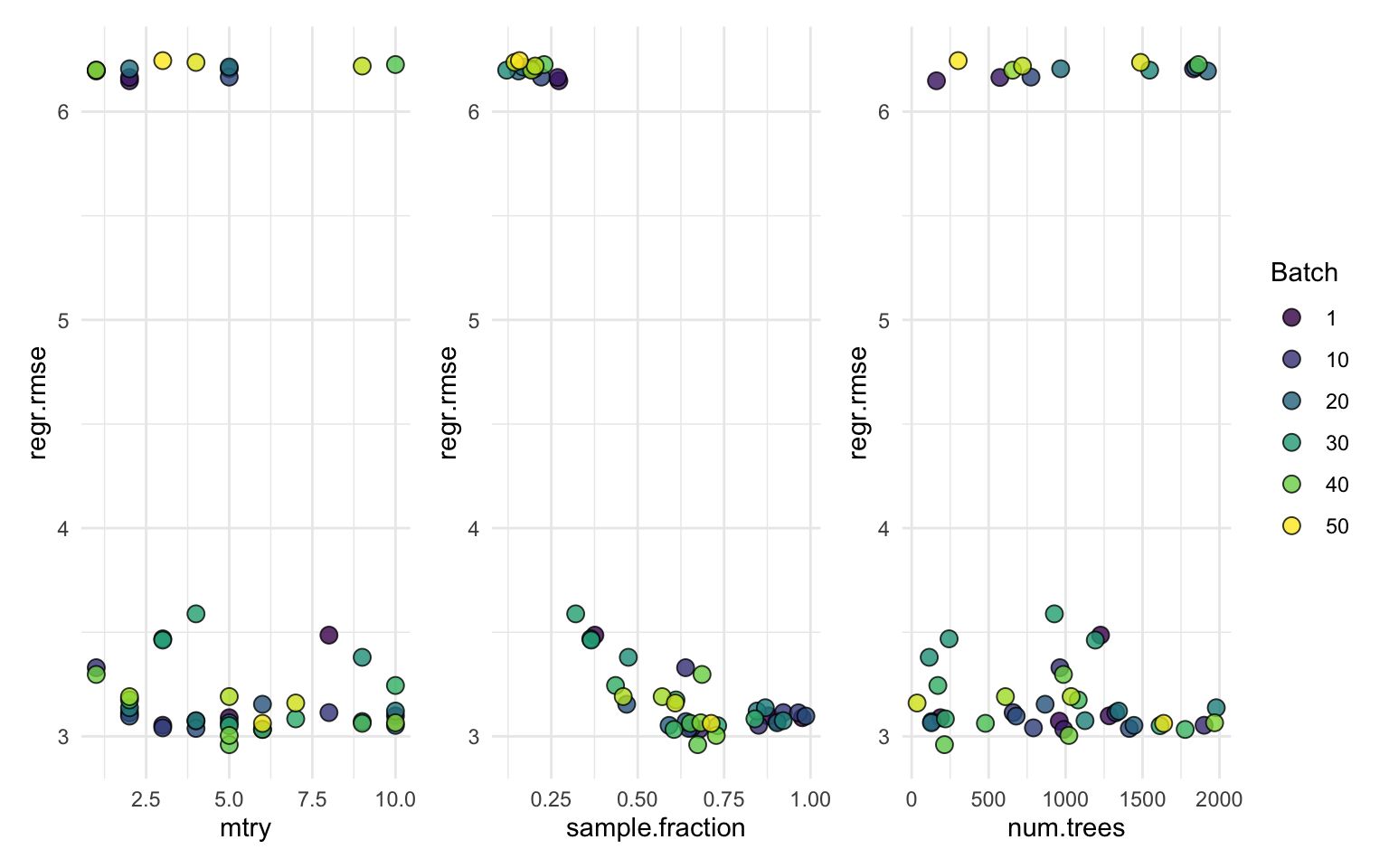
As during the HPO stage, I used 3-fold CV, the model has not seen the full data all at once. So, now I’ll train the model using the optimised hyperparameters.
lrn_ranger_tuned <- lrn("regr.ranger")
lrn_ranger_tuned$param_set$values = instance$result_learner_param_vals
lrn_ranger_tuned$train(tsk_mtcars)$model
Warning in .__Task__weights(self = self, private = private, super = super, : 'Task$weights' is deprecated.
Use 'Task$weights_learner' instead.
See help("Deprecated")Ranger result
Call:
ranger::ranger(dependent.variable.name = task$target_names, data = task$data(), case.weights = task$weights$weight, mtry = 5L, num.threads = 1L, num.trees = 128L, sample.fraction = 0.903474943945184)
Type: Regression
Number of trees: 128
Sample size: 32
Number of independent variables: 10
Mtry: 5
Target node size: 5
Variable importance mode: none
Splitrule: variance
OOB prediction error (MSE): 5.428537
R squared (OOB): 0.8505527 I tuned the regr.ranger learner on the mtcars dataset, focusing on three hyperparameters:
mtry: number of variables considered at each split,num.trees: number of trees in the forest,sample.fraction: fraction of the dataset used for each tree.Steps I took:
Exploration I inspected the available parameters for the learner using $param_set.
Learner setup I defined the tuning ranges with to_tune():
mtry from 1 to 10,num.trees from 1 to 100,000,sample.fraction from 0.1 to 1.Tuning instance I created a TuningInstanceSingleCrit using:
mtcars task,Running the tuner I used tnr("random_search") and called $optimize() to run the search. I then extracted the best hyperparameter combination and the archive of evaluated configurations.
Visualising results I used marginal plots to visualise the effect of each hyperparameter on the cross-validated RMSE.
Training the final model I retrained the regr.ranger model on the full dataset using the best parameters found.
Evaluate the performance of the model created in Exercise 1 with nested resampling. Use a holdout validation for the inner resampling and a 3-fold CV for the outer resampling.
OK, so here we need an outer and inner resampling strategy. The outer resampling strategy will be a 3-fold CV, and the inner resampling strategy will be a holdout validation.

Figure 1 shows an example of a nest resampling strategy (with 3-fold CV on the outer and 4-fold CV on the inner nest). Here, we need to do something slightly different as we are using the holdout resampling strategy on the inner nest.
I will use AutoTuner to do nested resampling, as that is what is done in Section 4.3.1 of the mlr3 tutorial.
## create auto_tuner to resample a random forest
# with 3-fold CV in outer resampling and
# holdout validation in inner resampling
at <- auto_tuner(
tuner = tnr("random_search"),
learner = lrn("regr.ranger",
mtry = to_tune(1, 1e1),
num.trees = to_tune(1, 1e5),
sample.fraction = to_tune(0.1, 1)),
# inner resampling
resampling = rsmp("holdout", ratio = 0.7),
measure = msr("regr.rmse"),
terminator = trm("evals", n_evals = 50)
)
# resampling step
rr <- resample(tsk("mtcars"),
at,
# outer resampling
rsmp("cv", folds = 3),
store_models = TRUE)
rrstore_models = TRUE so that the AutoTuner models (fitted on the outer training data) are stored,
── <ResampleResult> with 3 resampling iterations ───────────────────────────────
 task_id        learner_id resampling_id iteration  prediction_test warnings
  mtcars regr.ranger.tuned            cv         1 <PredictionRegr>        0
  mtcars regr.ranger.tuned            cv         2 <PredictionRegr>        0
  mtcars regr.ranger.tuned            cv         3 <PredictionRegr>        0
 errors
      0
      0
      0
Now I aggregate across the three outer folds to get the final performance.
rr$aggregate()regr.mse
13.13362 The inner tuning results can also be accessed, returning the optimal configurations (across all outer folds) and the full tuning archives.
# optimal configurations
extract_inner_tuning_results(rr)
iteration mtry num.trees sample.fraction regr.rmse learner_param_vals
<int> <int> <int> <num> <num> <list>
1: 1 1 81784 0.6769030 2.884958 <list[4]>
2: 2 5 73924 0.9194928 2.065022 <list[4]>
3: 3 3 15719 0.7797092 1.807826 <list[4]>
x_domain task_id learner_id resampling_id
<list> <char> <char> <char>
1: <list[3]> mtcars regr.ranger.tuned cv
2: <list[3]> mtcars regr.ranger.tuned cv
3: <list[3]> mtcars regr.ranger.tuned cv# full tuning archives
extract_inner_tuning_archives(rr) iteration mtry num.trees sample.fraction regr.rmse x_domain_mtry
<int> <int> <int> <num> <num> <int>
1: 1 2 15547 0.3219244 5.115809 2
2: 1 8 23468 0.3020848 5.113502 8
3: 1 5 47564 0.3500007 5.115646 5
4: 1 9 14922 0.8105999 3.261807 9
5: 1 2 81447 0.1308460 5.124990 2
---
146: 3 5 20556 0.5608060 2.081965 5
147: 3 2 9179 0.8461799 1.867438 2
148: 3 4 93847 0.1486419 3.733662 4
149: 3 3 15719 0.7797092 1.807826 3
150: 3 1 31967 0.2513883 3.739324 1
x_domain_num.trees x_domain_sample.fraction runtime_learners
<int> <num> <num>
1: 15547 0.3219244 0.055
2: 23468 0.3020848 0.096
3: 47564 0.3500007 0.208
4: 14922 0.8105999 0.110
5: 81447 0.1308460 0.372
---
146: 20556 0.5608060 0.120
147: 9179 0.8461799 0.054
148: 93847 0.1486419 0.398
149: 15719 0.7797092 0.097
150: 31967 0.2513883 0.118
timestamp warnings errors batch_nr resample_result task_id
<POSc> <int> <int> <int> <list> <char>
1: 2025-10-14 20:20:12 0 0 1 <ResampleResult> mtcars
2: 2025-10-14 20:20:12 0 0 2 <ResampleResult> mtcars
3: 2025-10-14 20:20:12 0 0 3 <ResampleResult> mtcars
4: 2025-10-14 20:20:12 0 0 4 <ResampleResult> mtcars
5: 2025-10-14 20:20:12 0 0 5 <ResampleResult> mtcars
---
146: 2025-10-14 20:20:54 0 0 46 <ResampleResult> mtcars
147: 2025-10-14 20:20:54 0 0 47 <ResampleResult> mtcars
148: 2025-10-14 20:20:55 0 0 48 <ResampleResult> mtcars
149: 2025-10-14 20:20:55 0 0 49 <ResampleResult> mtcars
150: 2025-10-14 20:20:55 0 0 50 <ResampleResult> mtcars
learner_id resampling_id
<char> <char>
1: regr.ranger.tuned cv
2: regr.ranger.tuned cv
3: regr.ranger.tuned cv
4: regr.ranger.tuned cv
5: regr.ranger.tuned cv
---
146: regr.ranger.tuned cv
147: regr.ranger.tuned cv
148: regr.ranger.tuned cv
149: regr.ranger.tuned cv
150: regr.ranger.tuned cvI evaluated the performance of the tuned model using nested resampling to obtain an unbiased estimate.
Steps I took:
Resampling strategy I used:
AutoTuner setup I reused the same regr.ranger learner and parameter ranges as in Question 1, wrapped in an AutoTuner. The tuning again used 50 evaluations of random search and MSE as the measure.
Resample execution I called resample() with the outer CV and the AutoTuner, setting store_models = TRUE to keep the fitted models from each outer fold.
Aggregating performance I used $aggregate() to average the MSE across the outer test folds.
Inspecting inner results I extracted the best configurations and full tuning logs from each inner loop using extract_inner_tuning_results() and extract_inner_tuning_archives().
Tune and benchmark an XGBoost model against a logistic regression (without tuning the latter) and determine which has the best Brier score. Use mlr3tuningspaces and nested resampling, try to pick appropriate inner and outer resampling strategies that balance computational efficiency vs. stability of the results.
I’ll use the built-in spam task – since the outcome is categorical, this is a classification task.
tsk_spam <- tsk("spam")First I’ll set up the logistic regression model (with no tuning).
# requires probs to compute the brier score
lrn_logreg <- lrn("classif.log_reg", predict_type = "prob")
The XGBoost model has lots of hyperparameters:
lrn("classif.xgboost")$param_set$ids() [1] "alpha" "approxcontrib"
[3] "base_score" "booster"
[5] "callbacks" "colsample_bylevel"
[7] "colsample_bynode" "colsample_bytree"
[9] "device" "disable_default_eval_metric"
[11] "early_stopping_rounds" "eta"
[13] "eval_metric" "feature_selector"
[15] "gamma" "grow_policy"
[17] "interaction_constraints" "iterationrange"
[19] "lambda" "lambda_bias"
[21] "max_bin" "max_delta_step"
[23] "max_depth" "max_leaves"
[25] "maximize" "min_child_weight"
[27] "missing" "monotone_constraints"
[29] "nrounds" "normalize_type"
[31] "nthread" "ntreelimit"
[33] "num_parallel_tree" "objective"
[35] "one_drop" "outputmargin"
[37] "predcontrib" "predinteraction"
[39] "predleaf" "print_every_n"
[41] "process_type" "rate_drop"
[43] "refresh_leaf" "reshape"
[45] "seed_per_iteration" "sampling_method"
[47] "sample_type" "save_name"
[49] "save_period" "scale_pos_weight"
[51] "skip_drop" "strict_shape"
[53] "subsample" "top_k"
[55] "training" "tree_method"
[57] "tweedie_variance_power" "updater"
[59] "verbose" "watchlist"
[61] "xgb_model" The main ones are:
| Hyperparameter | Description | Type |
|---|---|---|
eta |
Learning rate (shrinkage) | numeric |
max_depth |
Maximum depth of trees | integer |
nrounds |
Number of boosting rounds (trees) | integer |
colsample_bytree |
Fraction of features randomly sampled per tree | numeric |
subsample |
Fraction of rows sampled per tree | numeric |
min_child_weight |
Minimum sum of instance weights in a child node | numeric |
gamma |
Minimum loss reduction to make a split | numeric |
lambda |
L2 regularisation term on weights | numeric |
alpha |
L1 regularisation term on weights | numeric |
A typical tuning strategy for XGBoost might involve:
max_depthetanroundssubsamplecolsample_bytreemin_child_weightgammalambda (L2)alpha (L1)For the XGBoost learner, I’m going to use a predefined search space from {mlr3tuningspaces}. First, I’ll give a list of these predefined spaces.
mlr_tuning_spaces$keys()[grepl("xgboost", mlr_tuning_spaces$keys())][1] "classif.xgboost.default" "classif.xgboost.rbv1"
[3] "classif.xgboost.rbv2" "regr.xgboost.default"
[5] "regr.xgboost.rbv1" "regr.xgboost.rbv2" I will use the classif.xgboost.default space.
space = lts("classif.xgboost.default")
space
<TuningSpace:classif.xgboost.default>: Classification XGBoost with Default
id lower upper levels logscale
<char> <num> <num> <list> <lgcl>
1: eta 1e-04 1 [NULL] TRUE
2: nrounds 1e+00 5000 [NULL] FALSE
3: max_depth 1e+00 20 [NULL] FALSE
4: colsample_bytree 1e-01 1 [NULL] FALSE
5: colsample_bylevel 1e-01 1 [NULL] FALSE
6: lambda 1e-03 1000 [NULL] TRUE
7: alpha 1e-03 1000 [NULL] TRUE
8: subsample 1e-01 1 [NULL] FALSEPlugging this into auto_tuner() creates an AutoTuner object. I’m going to use 5-fold CV in the inner resampling and a terminator based on run time (of 60 seconds).
# create terminator with time budget of 60 secs
trm_rt = trm("run_time")
trm_rt$param_set$values$secs = 60

# create xgboost learner with prob predict_type
# 'prob' required for brier score
lrn_xgb = lrn("classif.xgboost", predict_type = "prob")

at_xgb <- auto_tuner(learner = lrn_xgb,
                    resampling = rsmp("cv", folds = 5),
                    measure = msr("classif.bbrier"),
                    terminator = trm_rt,
                    tuner = tnr("random_search"),
                    search_space = space)
at_xgb
── <AutoTuner> (classif.xgboost.tuned) ─────────────────────────────────────────
• Model: list
• Parameters: list()
• Packages: mlr3, mlr3tuning, mlr3learners, and xgboost
• Predict Types: response and [prob]
• Feature Types: logical, integer, and numeric
• Encapsulation: none (fallback: -)
• Properties: hotstart_forward, importance, missings, multiclass, offset,
twoclass, and weights
• Other settings: use_weights = 'use'
* Search Space:
                  id    class     lower       upper nlevels
              <char>   <char>     <num>       <num>   <num>
1:             alpha ParamDbl -6.907755    6.907755     Inf
2: colsample_bylevel ParamDbl  0.100000    1.000000     Inf
3:  colsample_bytree ParamDbl  0.100000    1.000000     Inf
4:               eta ParamDbl -9.210340    0.000000     Inf
5:            lambda ParamDbl -6.907755    6.907755     Inf
6:         max_depth ParamInt  1.000000   20.000000      20
7:           nrounds ParamInt  1.000000 5000.000000    5000
8:         subsample ParamDbl  0.100000    1.000000     Inf
Now I can set up the outer resampling strategy (4-fold CV).
outer_rsmp <- rsmp("cv", folds = 4)I can create a benchmark grid and run it for the task to compare the two learners.
# Benchmark both learners
design = benchmark_grid(
  tasks = tsk_spam,
  learners = list(lrn_logreg, at_xgb),
  resamplings = outer_rsmp
)
design
task learner resampling
<char> <char> <char>
1: spam classif.log_reg cv
2: spam classif.xgboost.tuned cv# run the benchmark design
set.seed(101)
bmr = benchmark(design)Warning: glm.fit: fitted probabilities numerically 0 or 1 occurred
Warning: glm.fit: fitted probabilities numerically 0 or 1 occurred
Warning: glm.fit: fitted probabilities numerically 0 or 1 occurred
Warning: glm.fit: fitted probabilities numerically 0 or 1 occurred# the score for each of the 4-fold CV outer folds
bmr$score(msr("classif.bbrier"))[,
.(learner_id, resampling_id, iteration, classif.bbrier)
] learner_id resampling_id iteration classif.bbrier
<char> <char> <int> <num>
1: classif.log_reg cv 1 0.06236199
2: classif.log_reg cv 2 0.05802780
3: classif.log_reg cv 3 0.05744753
4: classif.log_reg cv 4 0.05651042
5: classif.xgboost.tuned cv 1 0.04560204
6: classif.xgboost.tuned cv 2 0.02618333
7: classif.xgboost.tuned cv 3 0.04326268
8: classif.xgboost.tuned cv 4 0.03606656# the aggregate score for each learner
bmr$aggregate(msr("classif.bbrier"))[,
.(learner_id, resampling_id, classif.bbrier)
] learner_id resampling_id classif.bbrier
<char> <char> <num>
1: classif.log_reg cv 0.05858693
2: classif.xgboost.tuned cv 0.03777865I can use autoplot to plot these results.
autoplot(bmr, measure = msr("classif.bbrier"))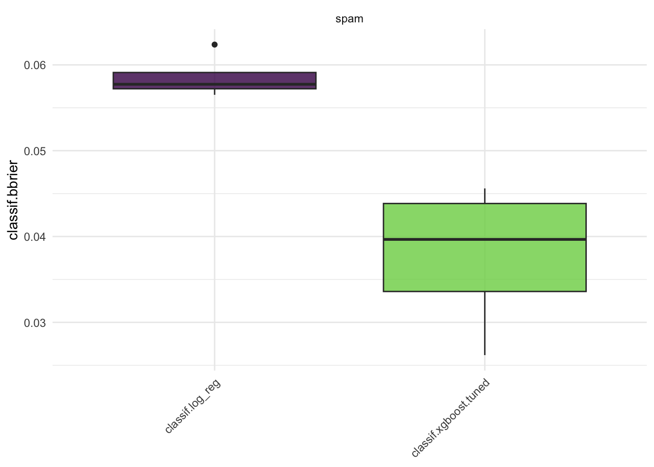
So, XGBoost performs better than the logistic regression model on the spam task. But, the XGBoost model is much more computationally expensive, takes longer to train, and is less interpretable. So, the choice of model is a trade off between performance and interpretability.
I benchmarked a tuned XGBoost model against an untuned logistic regression model on the spam classification task using the Brier score.
Steps I took:
Loading the task
I used the built-in tsk("spam").
Logistic regression setup
I defined a classif.log_reg learner with predict_type = "prob" to enable Brier score calculation.
XGBoost setup with tuning
I used classif.xgboost with predict_type = "prob" and the predefined tuning space lts("classif.xgboost.default") from {mlr3tuningspaces}.
AutoTuner for XGBoost
I created an AutoTuner with:
trm("run_time"),Outer resampling
I used 4-fold CV for the outer loop.
Benchmark setup and execution
I created a benchmark grid comparing both learners on the task, ran the benchmark, and scored the results using the Brier score.
Results
I looked at individual fold scores using bmr$score() and aggregate performance using bmr$aggregate(). I also visualised the comparison with autoplot().
Write a function that implements an iterated random search procedure that drills down on the optimal configuration by applying random search to iteratively smaller search spaces. Your function should have seven inputs: task, learner, search_space, resampling, measure, random_search_stages, and random_search_size. You should only worry about programming this for fully numeric and bounded search spaces that have no dependencies. In pseudo-code:
a. Create a random design of size `random_search_size` from the given search space and evaluate the learner on it.
b. Identify the best configuration.
c. Create a smaller search space around this best config, where you define the new range for each parameter as: `new_range[i] = (best_conf[i] - 0.25 * current_range[i], best_conf[i] + 0.25*current_range[i])`. Ensure that this `new_range` respects the initial bound of the original `search_space` by taking the `max()` of the new and old lower bound, and the `min()` of the new and the old upper bound (“clipping”).
d. Iterate the previous steps `random_search_stages` times and at the end return the best configuration you have ever evaluated. As a stretch goal, look into `mlr3tuning`’s internal source code and turn your function into an R6 class inheriting from the `TunerBatch` class – test it out on a learner of your choice.mtcars datasetLet’s start by trying this out on the mtcars dataset, using the regr.rpart learner. I’ll make it simpler by using the to_tune() function, which means I don’t have to define the search space manually to be e.g. an integer, double etc..
First, I’ll load the task and learner, and then look at the hyperparameters of this learner.
task <- tsk("mtcars")
learner <- lrn("regr.rpart")
# look at the hyperparameters
as.data.table(learner$param_set)[, .(id, class, lower, upper)]
id class lower upper
<char> <char> <num> <num>
1: cp ParamDbl 0 1
2: keep_model ParamLgl NA NA
3: maxcompete ParamInt 0 Inf
4: maxdepth ParamInt 1 30
5: maxsurrogate ParamInt 0 Inf
6: minbucket ParamInt 1 Inf
7: minsplit ParamInt 1 Inf
8: surrogatestyle ParamInt 0 1
9: usesurrogate ParamInt 0 2
10: xval ParamInt 0 Inf| ID | Description | Typical Range | Notes |
|---|---|---|---|
cp |
Complexity parameter: controls cost of adding splits | [0.001, 0.1] (log-scale) | Lower values allow deeper trees |
maxdepth |
Maximum depth of the tree | 1–30 | Prevents trees from growing too deep |
minsplit |
Minimum number of observations required to attempt a split | 2–20 | Higher values make trees more conservative |
minbucket |
Minimum number of observations in any terminal node | 1–10 | If not set, defaults to minsplit / 3 |
Part 1: creating a search_space and evaluating the learner
I’ll now create a search space to tune the four hyperparameters cp, maxdepth, minsplit, and minbucket, using to_tune().
# use to_tune() to create the search space
learner$param_set$values$cp <- to_tune(1e-4, 0.1)
learner$param_set$values$maxdepth <- to_tune(1, 30)
learner$param_set$values$minsplit <- to_tune(2, 20)
learner$param_set$values$minbucket <- to_tune(1, 10)

param_ids <- names(Filter(function(x) inherits(x, "TuneToken"), learner$param_set$values))
# filter param_set bu param_names
learner$param_set$values[param_ids]
$cp
Tuning over:
range [1e-04, 0.1]
$maxdepth
Tuning over:
range [1, 30]
$minbucket
Tuning over:
range [1, 10]
$minsplit
Tuning over:
range [2, 20]Now I’ll tune the learner on this search space using a random search with 50 evaluations and 3-fold CV.
# create random search tuner
tuner <- tnr("random_search")
# create measure
measure <- msr("regr.rmse")
# create resampling strategy
resampling <- rsmp("cv", folds = 3)
# create terminator
terminator <- trm("evals", n_evals = 50)
# create tuning instance and run tuner
set.seed(333)
instance <- mlr3tuning::tune(
tuner = tuner,
task = task,
learner = learner,
resampling = resampling,
measure = measure,
terminator = terminator
)tune() - the one from {mlr3tuning} instead of from {e1701}. If the latter is used, you get an error like argument "train.x" is missing, with no default.
Part 2: Identifying the best configuration
We can see the result be looking at the instance object.
instance
── <TuningInstanceBatchSingleCrit> ─────────────────────────────────────────────
• State: Optimized
• Objective: <ObjectiveTuningBatch>
• Search Space:
          id    class lower upper nlevels
      <char>   <char> <num> <num>   <num>
1:        cp ParamDbl 1e-04   0.1     Inf
2:  maxdepth ParamInt 1e+00  30.0      30
3: minbucket ParamInt 1e+00  10.0      10
4:  minsplit ParamInt 2e+00  20.0      19
• Terminator: <TerminatorEvals> (n_evals=50, k=0)
• Result:
           cp maxdepth minbucket minsplit regr.rmse
        <num>    <int>     <int>    <int>     <num>
1: 0.02942214       18         3        5  3.488251
• Archive:
    regr.rmse    cp maxdepth minbucket minsplit
        <num> <num>    <int>     <int>    <int>
 1:         4 0.033       30         1        6
 2:         4 0.041       30         7       17
 3:         4 0.043       26        10       15
 4:         4 0.039        1        10        3
 5:         4 0.043        2         9        7
---
46:         4 0.076        3         9        9
47:         3 0.063       16         3        4
48:         4 0.008        2         3       11
49:         4 0.082       18         3       10
50:         4 0.018       12         5        7
The best configuration is stored in the result_learner_param_vals slot of the instance object.
# get the best configuration
best_config1 <- instance$result_learner_param_vals[param_ids]
unlist(best_config1)
cp maxdepth minbucket minsplit
0.02942214 18.00000000 3.00000000 5.00000000 The root mean-squared error is stored in instance$result_y:
# get the RMSE
best_rmse1 <- instance$result_y
best_rmse1
regr.rmse
3.488251 Part 3: create a smaller search space around the best configuration
# obtain new upper and lower bounds
# helper function to adjust bounds

adjust_bounds <- function(param_id, best_config, learner, shrink = 0.25) {
  param = learner$param_set$values[[param_id]]$content
  bounds = list(lower = param$lower, upper = param$upper)
  best = best_config[[param_id]]
  range = bounds$upper - bounds$lower
  lower_bound <- best - shrink * range
  upper_bound <- best + shrink * range
  # if class is ParamInt, then set lower to be ceiling and upper to be floor
  # obtain class of the parameter
  param_class <- learner$param_set$params[id == param_id, setNames(cls, id)]
  if (param_class == "ParamInt") {
    lower_bound = ceiling(lower_bound)
    upper_bound = floor(upper_bound)
  }
  lower_new = max(lower_bound, bounds$lower)
  upper_new = min(upper_bound, bounds$upper)
  list(lower = lower_new, upper = upper_new)
}

adjusted_bounds <- lapply(param_ids,
                          adjust_bounds,
                          best_config = best_config1,
                          learner = learner)

names(adjusted_bounds) <- param_ids

# update learner
learner$param_set$values$cp <- to_tune(adjusted_bounds$cp$lower,
                                       adjusted_bounds$cp$upper)
learner$param_set$values$maxdepth <- to_tune(adjusted_bounds$maxdepth$lower,
                                             adjusted_bounds$maxdepth$upper)
learner$param_set$values$minsplit <- to_tune(adjusted_bounds$minsplit$lower,
                                             adjusted_bounds$minsplit$upper)
learner$param_set$values$minbucket <- to_tune(adjusted_bounds$minbucket$lower,
                                              adjusted_bounds$minbucket$upper)
# check the new search space
Filter(function(x) inherits(x, "TuneToken"), learner$param_set$values)
$cp
Tuning over:
range [0.00444714480435941, 0.0543971448043594]
$maxdepth
Tuning over:
range [11, 25]
$minbucket
Tuning over:
range [1, 5]
$minsplit
Tuning over:
range [2, 9]Part 4: evaluate the learner on the new search space
# create new tuning instance and run tuner
set.seed(222)
instance <- mlr3tuning::tune(
  tuner = tuner,
  task = task,
  learner = learner,
  resampling = resampling,
  measure = measure,
  terminator = terminator
)
Get the best configuration from this:
# get the best configuration
best_config2 <- instance$result_learner_param_vals[param_ids]
unlist(best_config2)
cp maxdepth minbucket minsplit
0.01176303 15.00000000 1.00000000 4.00000000 and the RMSE:
# get the RMSE
best_rmse2 <- instance$result_y
best_rmse2
regr.rmse
3.724687 Cool, so I have a new best configuration. Does it perform better than the first?
# Best configuration from the first tuning
best_config1
$cp
[1] 0.02942214
$maxdepth
[1] 18
$minbucket
[1] 3
$minsplit
[1] 5# RMSE from the first configuration
best_rmse1regr.rmse
3.488251 # Best configuration from the second tuning
best_config2$cp
[1] 0.01176303
$maxdepth
[1] 15
$minbucket
[1] 1
$minsplit
[1] 4# RMSE from the second configuration
best_rmse2regr.rmse
3.724687 # compare the two RMSEs
best_rmse2 - best_rmse1regr.rmse
0.236436 No, it doesn’t. I can repeat this process iteratively on smaller subspaces. At the end, choose the best configuration by selecting the one with the lowest RMSE.
The next step is to create a function that does this for me.
So, this function has the following inputs: - task: the task to tune; - learner: the learner to tune; - search_space: the search space to tune; - this should be a data.table of the hyperparameters to tune, with class, and the lower and upper bounds; - resampling: the resampling strategy to use; - measure: the measure to use; - random_search_stages: the number of random search stages to perform; - random_search_size: the number of random evaluations to perform in each stage.
The function will return the best configuration found across all stages.
First, I created a checker function to make sure all the inputs are valid.2
2 Actually I created this last, but it’s required before my function so I’ll put it here
.inputChecks <- function(task, learner, search_space, resampling, measure,
                         random_search_stages, random_search_size) {

        ## error checking
        # check input classes
        stopifnot(inherits(task, "Task"))
        stopifnot(inherits(learner, "Learner"))
        stopifnot(inherits(resampling, "Resampling"))
        stopifnot(inherits(measure, "Measure"))
        # check search space: required columns exist and are numeric where needed
        required_cols <- c("id", "lower", "upper")
        missing_cols <- setdiff(required_cols, colnames(search_space))
        if (length(missing_cols) > 0) {
          stop("search_space must contain columns: ", paste(missing_cols, collapse = ", "))
        }

        if (!all(sapply(search_space[, .(lower, upper)], is.numeric))) {
          stop("Columns 'lower' and 'upper' in search_space must be numeric")
        }
        # check ids match those in learner
        invalid_ids <- setdiff(search_space$id, learner$param_set$ids())
        if (length(invalid_ids) > 0) {
          stop("Invalid parameter IDs in search_space: ", paste(invalid_ids, collapse = ", "))
        }
        # check iterations inputs
        stopifnot(is.numeric(random_search_stages), random_search_stages >= 1)
        stopifnot(is.numeric(random_search_size), random_search_size >= 1)
}
Now, let’s create the function.
iterative_random_tuner <- function(task, learner, search_space,
                                   resampling, measure,
                                   random_search_stages, random_search_size,
                                   verbose = TRUE, seed = TRUE) {

  .inputChecks(task, learner, search_space, resampling, measure,
               random_search_stages, random_search_size)

  param_ids <- search_space$id
  tuner <- tnr("random_search")
  terminator <- trm("evals", n_evals = random_search_size)

  # initialise search space on learner
  learner$param_set$values[param_ids] <- Map(to_tune,
                                             search_space$lower,
                                             search_space$upper)

  best_config_list <- list()

  if (seed) set.seed(22)
  for (stage in seq_len(random_search_stages)) {
    if (stage > 1) {
      # update search space based on previous best
      adjusted_bounds <- lapply(param_ids, adjust_bounds,
                                best_config = best_config,
                                learner = learner)
      names(adjusted_bounds) <- param_ids
      learner$param_set$values[param_ids] <- Map(to_tune,
                                                 lapply(adjusted_bounds, `[[`, "lower"),
                                                 lapply(adjusted_bounds, `[[`, "upper"))
    }

    # tune
    instance <- mlr3tuning::tune(
      tuner = tuner,
      task = task,
      learner = learner,
      resampling = resampling,
      measure = measure,
      terminator = terminator
    )

    best_config <- unlist(instance$result_learner_param_vals[param_ids])
    best_score <- instance$result_y

    best_config_list[[stage]] <- list(config = best_config, score = best_score)

    if (verbose) cat(sprintf("Stage %d score: %.3f\n", stage, best_score))
  }

  # label the list
  names(best_config_list) <- paste0("stage_", seq_along(best_config_list))

  # return best config only
  best_index <- if (measure$minimize) {
    which.min(sapply(best_config_list, `[[`, "score"))
  } else {
    which.max(sapply(best_config_list, `[[`, "score"))
  }

  best_config_list[[best_index]]
}
Now I can run this function on the mtcars dataset.
# create search space
search_space <- rbindlist(list(
  list(id = "cp", lower = 1e-4, upper = 1),
  list(id = "maxdepth", lower = 1,    upper = 30),
  list(id = "minsplit", lower = 2,    upper = 20),
  list(id = "minbucket", lower = 1,   upper = 10)
))

best_config <- iterative_random_tuner(
        task = task,
        learner = learner,
        search_space = search_space,
        resampling = rsmp("cv", folds = 3),
        measure = msr("regr.rmse"),
        random_search_stages = 5,
        random_search_size = 50
)
Stage 1 score: 3.515
Stage 2 score: 3.686
Stage 3 score: 3.573
Stage 4 score: 3.608
Stage 5 score: 4.212best_config$config
cp maxdepth minsplit minbucket
0.04672705 16.00000000 6.00000000 1.00000000
$score
regr.rmse
3.515434 Nice one.
Great. Let’s summarise what I’ve done in this post.
Exercise 1: Hyperparameter Tuning with Random Search
regr.ranger on mtcars datasetmtry, num.trees, sample.fractionExercise 2: Nested Resampling
AutoTuner with same hyperparameter setup as Q1Exercise 3: Benchmarking XGBoost vs Logistic Regression
spam datasetmlr3tuningspaces::lts("classif.xgboost.default")@online{smith2025,
author = {Smith, Paul and Smith, Paul},
title = {Getting {Started} with \{Mlr3\}},
date = {2025-03-21},
url = {https://pws3141.github.io/blog/posts/09-mlr3_hyperparameter/},
langid = {en}
}